LSQquad.m
Contents
Overview
Illustrates the effect of ill-conditioning of the normal equations by performing least squares solution in double and single-precision
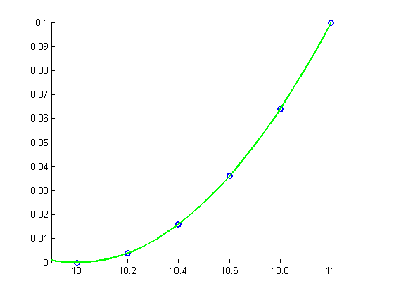
First Example: Solving the normal equations in double precision
clear all
close all
x = [10:0.2:11]';
y = [0:0.2:1]'.^2/10;
m = length(x);
hold on
plot(x, y, 'bo', 'LineWidth',2)
xlim([9.9 11.1])
ylim([0 0.1])
pause
disp('Using double-precision')
A = [x.^2 x ones(m,1)]
% Solve the normal equations
c = (A'*A)\(A'*y)
xx = linspace(9.9,11.1,50);
yy = c(1)*xx.^2+c(2)*xx+c(3);
plot(xx, yy, 'g-', 'LineWidth', 2)
hold off
Using double-precision

A =

  100.0000   10.0000    1.0000
  104.0400   10.2000    1.0000
  108.1600   10.4000    1.0000
  112.3600   10.6000    1.0000
  116.6400   10.8000    1.0000
  121.0000   11.0000    1.0000


c =

    0.1000
   -2.0000
   10.0000
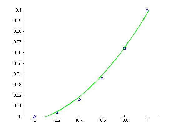
Second Example: Solving the normal equations in single precision
We will find out that the problem lies with the condition number of the normal equations matrix  , which is roughly the square of the condition number of
  .
.
pause
disp('Using single-precision')
figure
hold on
plot(x, y, 'bo', 'LineWidth',2)
xlim([9.9 11.1])
ylim([0 0.1])
A = [single(x.^2) x ones(m,1)];
% Solve the normal equations
c = single((A'*A))\single((A'*y))
xx = linspace(9.9,11.1,50);
yy = c(1)*xx.^2+c(2)*xx+c(3);
plot(xx, yy, 'g-', 'LineWidth', 2)
hold off
pause
disp(sprintf('The problem lies with the condition number of A^TA.\n cond(A^TA) = %e\n',cond(A'*A)))
disp(sprintf('For comparison, cond(A) = %e\n',cond(A)))
Using single-precision
Warning: Matrix is close to singular or badly scaled.
         Results may be inaccurate. RCOND = 6.867955e-011.

c =

    0.0751
   -1.4762
    7.2522

The problem lies with the condition number of A^TA.
 cond(A^TA) = 1.179585e+010

For comparison, cond(A) = 1.248895e+005
Third Example: Again in single precision, but using a more stable method
pause
disp('Solution using a more stable method (also in single-precision)')
figure
hold on
plot(x, y, 'bo', 'LineWidth',2)
xlim([9.9 11.1])
ylim([0 0.1])
A = [single(x.^2) x ones(m,1)];
% Solve the overdetermined system directly via backslash (implicitly, this
% corresponds to a QR decomposition)
c = A\single(y)
xx = linspace(9.9,11.1,50);
yy = c(1)*xx.^2+c(2)*xx+c(3);
plot(xx, yy, 'g-', 'LineWidth', 2)
hold off
Solution using a more stable method (also in single-precision)

c =

    0.1000
   -1.9999
    9.9997
