LSQquadOrtho.m
Contents
Overview
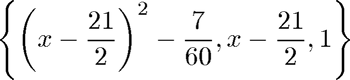
Illustrates the use of an orthogonal basis for the computation of a polynomial least squares fit
Solving the normal equations in single precision using an orthogonal basis
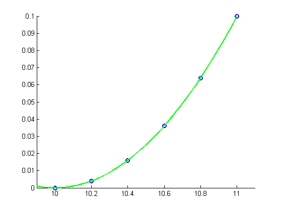
clear all
close all
x = [10:0.2:11]';
y = [0:0.2:1]'.^2/10;
m = length(x);
hold on
plot(x, y, 'bo', 'LineWidth',2)
xlim([9.9 11.1])
ylim([0 0.1])
pause
disp('Using single-precision with orthogonal basis')
A = [single((x-21/2).^2-7/60) single(x-21/2) ones(m,1)]
% Solve the normal equations
c = single((A'*A))\single((A'*y))
xx = linspace(9.9,11.1,50);
yy = c(1)*((xx-21/2).^2-7/60)+c(2)*(xx-21/2)+c(3);
plot(xx, yy, 'g-', 'LineWidth', 2)
hold off
disp(sprintf('There no longer is a problem with the condition number of A^TA.'))
disp(sprintf('cond(A^TA) = %e\n',cond(A'*A)))
disp(sprintf('For comparison, cond(A) = %e\n',cond(A)))
Using single-precision with orthogonal basis

A =

    0.1333   -0.5000    1.0000
   -0.0267   -0.3000    1.0000
   -0.1067   -0.1000    1.0000
   -0.1067    0.1000    1.0000
   -0.0267    0.3000    1.0000
    0.1333    0.5000    1.0000


c =

    0.1000
    0.1000
    0.0367

There no longer is a problem with the condition number of A^TA.
cond(A^TA) = 1.004464e+002

For comparison, cond(A) = 1.002230e+001
Compute the inner products of the columns of  with each other to verify that is an orthogonal matrix.
pause
disp('Notice that the columns of A are orthogonal to each other:')
disp(sprintf('A(:,1)''*A(:,2) = % f',A(:,1)'*A(:,2)))
disp(sprintf('A(:,1)''*A(:,3) = % f',A(:,1)'*A(:,3)))
disp(sprintf('A(:,2)''*A(:,3) = % f',A(:,2)'*A(:,3)))
Notice that the columns of A are orthogonal to each other:
A(:,1)'*A(:,2) =  0.000000
A(:,1)'*A(:,3) =  0.000000
A(:,2)'*A(:,3) =  0.000000