LSQquadQR.m
Contents
Overview
Illustrates the use of the QR decomposition for the computation of a polynomial least squares fit
Example 1: Solving the least squares problem using QR decomposition
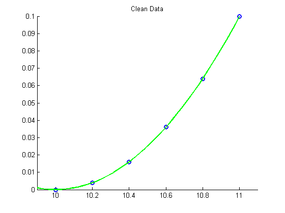
Data comes from the quadratic polynomial (no noise)
clear all
close all
x = [10:0.2:11]';
disp('Clean Data')
y = [0:0.2:1]'.^2/10;
m = length(x);
hold on
plot(x, y, 'bo', 'LineWidth',2)
xlim([9.9 11.1])
ylim([0 0.1])
%pause
disp('Solving least squares problem with QR decomposition')
A = [x.^2 x ones(m,1)]
% Compute the QR decomposition of A
[Q R] = qr(A)
Rhat = R(1:3,1:3)
z = Q(:,1:3)'*y;
c = Rhat\z
xx = linspace(9.9,11.1,50);
yy = c(1)*xx.^2+c(2)*xx+c(3);
plot(xx, yy, 'g-', 'LineWidth', 2)
title('Clean Data')
disp('Fitting with quadratic polynomial')
disp(sprintf('p(x) = %3.2fx^2 + %3.2fx + %3.2f',c))
hold off
Clean Data
Solving least squares problem with QR decomposition

A =

  100.0000   10.0000    1.0000
  104.0400   10.2000    1.0000
  108.1600   10.4000    1.0000
  112.3600   10.6000    1.0000
  116.6400   10.8000    1.0000
  121.0000   11.0000    1.0000


Q =

    0.3691    0.6074    0.5623   -0.1881   -0.0850   -0.3687
    0.3840    0.3872   -0.0987    0.5732    0.3351    0.5020
    0.3992    0.1579   -0.4326   -0.6543   -0.2266    0.3861
    0.4147   -0.0806   -0.4392    0.4051   -0.4804   -0.4834
    0.4305   -0.3282   -0.1187   -0.1994    0.7254   -0.3561
    0.4466   -0.5848    0.5291    0.0635   -0.2685    0.3201


R =

  270.9125   25.7197    2.4443
         0    0.8335    0.1589
         0         0    0.0022
         0         0         0
         0         0         0
         0         0         0


Rhat =

  270.9125   25.7197    2.4443
         0    0.8335    0.1589
         0         0    0.0022


c =

    0.1000
   -2.0000
   10.0000

Fitting with quadratic polynomial
p(x) = 0.10x^2 + -2.00x + 10.00
Example 2: Fit "noisy" data using a quadratic polynomial
Note that we do not need to re-compute the QR decomposition of the matrix  for this part since the matrix is still the same. Only the data vector
  has changed!
%pause
disp('Noisy Data')
% Add 10% noise to the data
y = y + 0.1*max(y)*rand(size(y));
figure
hold on
plot(x, y, 'bo', 'LineWidth',2)
xlim([9.9 11.1])
ylim([0 0.1])
%pause
disp('Solving noisy least squares problem with QR decomposition')
% No need to re-compute the QR decomposition of A since A is the same, only
% y has changed!
z = Q(:,1:3)'*y;
c = Rhat\z
xx = linspace(9.9,11.1,50);
yy = c(1)*xx.^2+c(2)*xx+c(3);
plot(xx, yy, 'g-', 'LineWidth', 2)
title('Noisy Data')
disp('Fitting with quadratic polynomial')
disp(sprintf('p(x) = %3.2fx^2 + %3.2fx + %3.2f',c))
hold off
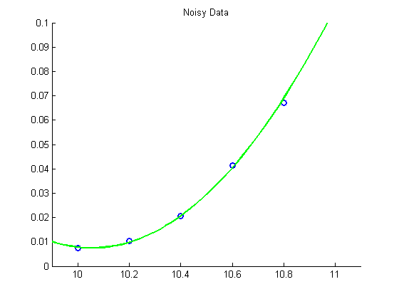
Noisy Data
Solving noisy least squares problem with QR decomposition

c =

    0.1109
   -2.2306
   11.2219

Fitting with quadratic polynomial
p(x) = 0.11x^2 + -2.23x + 11.22