LynxHareDemo.m
Contents
Overview
This script illustrates the solution of a system of first-order Lotka-Volterra (predator-prey) IVPs:
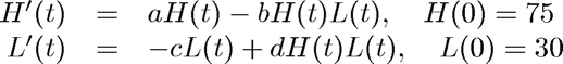
for finding the hare and lynx population (and to compare with the data recorded by the Hudson Bay Company).
Here  stands for time,
  and
and  stand for hare and lynx populations, and
 : birth rate of hares
 : death rate of hares, depends on interaction with lynx (how good are lynx at killing hares)
 : death rate of lynx
 : birth rate of lynx, depends on interaction with hares (how well do hares feed lynx)
The right-hand side function is coded in LynxHare.m
Initialization
clear all
clc
close all
f = @LynxHare;              % function handle for right-hand side function
t0 = 1855; y0 = [75; 30];   % initial time and initial population in thousands
tend = 1930;                % end time
N = 10000;                  % number of time steps
h = (tend-t0)/N;            % stepsize
Call Euler
We will discuss this function later
[t,y] = Euler(t0,y0,f,h,N);
We could also use a MATLAB ODE solver such as
[t,y] = ode23(f,[t0 tend],y0);
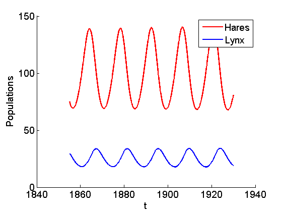
Plot
of the populations vs. time
figure
hold on
set(gca,'Fontsize',14)
xlabel('t','FontSize',14);
ylabel('Populations','FontSize',14);
plot(t,y(:,1),'r','LineWidth',2);    % hares
plot(t,y(:,2),'b','LineWidth',2);    % lynx
legend('Hares','Lynx');
hold off
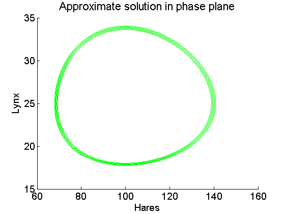
Plot of the populations in phase space
figure
hold on
title('Approximate solution in phase plane', 'Fontsize',16)
set(gca,'Fontsize',14)
xlabel('Hares','Fontsize',14)
ylabel('Lynx','Fontsize',14)
plot(y(:,1),y(:,2),'g','LineWidth',1);   % lynx vs. hares (phase plane)
hold off