QuadDemo.m
Contents
- Overview
- Inline functions are obsolete, so we no longer discuss their use.
- Integrand defined as anonymous function
- Integrand defined in external M-file besselintegrand.m
- Integrand defined as anonymous function with parameter
- Graphical illustration with quadgui
- An Experiment from NCM
- Other good examples for quadgui:
Overview
Illustrates the NCM routine quadtx (textbook version of quad) to perform numerical integration on the interval ![$[a, b]$](QuadDemo_eq40018.png) . Also illustrates different ways to define functions for use with function-functions.
. Also illustrates different ways to define functions for use with function-functions.
Inline functions are obsolete, so we no longer discuss their use.
Integrand defined as anonymous function
We evaluate
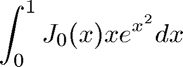
a = 0;
b = 1;
disp('Evaluate the complicated Bessel integral (f defined as anonymous function):')
f = @(x) besselj(0,x).*x.*exp(x.^2);
q = quadtx(f,a,b);
disp(sprintf('Int(J0(x)*x*exp(x^2),x=%f..%f) = %15.12f.\n',a,b,q))

%pause
Evaluate the complicated Bessel integral (f defined as anonymous function):
Int(J0(x)*x*exp(x^2),x=0.000000..1.000000) =  0.739631779804.
Integrand defined in external M-file besselintegrand.m
disp('Evaluate the complicated Bessel integral again (f defined in external M-file):')
q = quadtx(@besselintegrand,a,b);
disp(sprintf('Int(J0(x)*x*exp(x^2),x=%f..%f) = %15.12f.\n',a,b,q))

%pause
Evaluate the complicated Bessel integral again (f defined in external M-file):
Int(J0(x)*x*exp(x^2),x=0.000000..1.000000) =  0.739631779804.
Integrand defined as anonymous function with parameter
We now evaluate
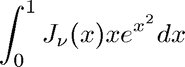
for values of 
disp('Evaluate even more complicated Bessel integrals:')
f = @(x,n) besselj(n,x).*x.*exp(x.^2);
for n=0:0.5:2
    % The fourth argument for quadtx expects a tolerance for the adaptive
    % subdivision. Even if we don't want to change it, we still need to
    % reserve space for it.
    q = quadtx(f,a,b,[],n);
    disp(sprintf('Int(J_%2.1f(x)*x*exp(x^2),x=%f..%f) = %15.12f.\n',n,a,b,q))
end

%pause
Evaluate even more complicated Bessel integrals:
Int(J_0.0(x)*x*exp(x^2),x=0.000000..1.000000) =  0.739631779804.

Int(J_0.5(x)*x*exp(x^2),x=0.000000..1.000000) =  0.518983492064.

Int(J_1.0(x)*x*exp(x^2),x=0.000000..1.000000) =  0.288627069603.

Int(J_1.5(x)*x*exp(x^2),x=0.000000..1.000000) =  0.137909969971.

Int(J_2.0(x)*x*exp(x^2),x=0.000000..1.000000) =  0.058849406764.
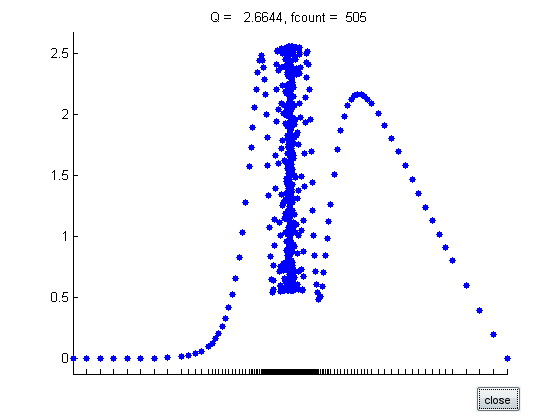
Graphical illustration with quadgui
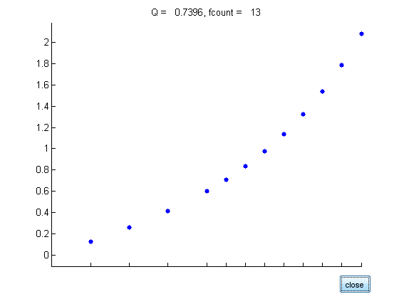
disp(sprintf('Now starting quadgui with Int(J_%2.1f(x)*x*exp(x^2),x=%f..%f)\n',n,a,b))
f = @(x) besselj(0,x).*x.*exp(x.^2);
q = quadgui(f,a,b);

%pause
Now starting quadgui with Int(J_2.0(x)*x*exp(x^2),x=0.000000..1.000000)
An Experiment from NCM
Modified to use the Bessel function integral
Qexact = 0.739631779338781;
%Qexact = 29.85832539549867;
disp('An experiment from NCM showing the effect of the tolerance')
disp('    tol              Q          fcount        err        ratio')
for k = 1:12
    tol = 10^(-k);
    [Q,fcount] = quadtx(f,0,1,tol);
%    [Q,fcount] = quadtx(@humps,0,1,tol);
    err = Q - Qexact;
    ratio = err/tol;
    fprintf('%8.0e %21.14f %7d %13.3e %9.3f\n', ...
        tol,Q,fcount,err,ratio)
end

%pause
An experiment from NCM showing the effect of the tolerance
    tol              Q          fcount        err        ratio
  1e-001      0.73974118141456       5    1.094e-004     0.001
  1e-002      0.73974118141456       5    1.094e-004     0.011
  1e-003      0.73963369998902       9    1.921e-006     0.002
  1e-004      0.73963212792942      13    3.486e-007     0.003
  1e-005      0.73963178505244      25    5.714e-009     0.001
  1e-006      0.73963177980438      33    4.656e-010     0.000
  1e-007      0.73963177936419      57    2.541e-011     0.000
  1e-008      0.73963177934112      89    2.339e-012     0.000
  1e-009      0.73963177933896     121    1.821e-013     0.000
  1e-010      0.73963177933879     221    7.550e-015     0.000
  1e-011      0.73963177933878     349    7.772e-016     0.000
  1e-012      0.73963177933878     485    2.220e-016     0.000
Other good examples for quadgui:
The humps function
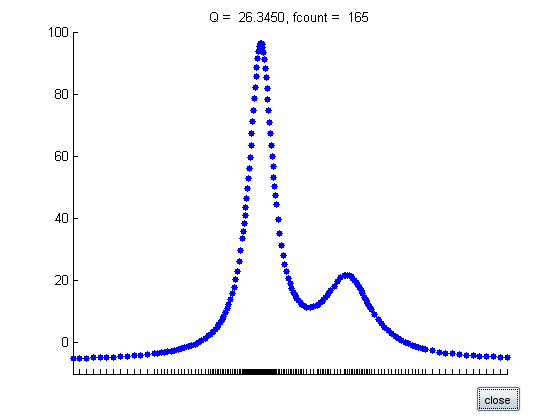
disp('Starting quadgui again with more examples')
disp('f(x) = humps(x) on [-1,2]')
f = @(x) humps(x);
a = -1; b = 2;
q = quadgui(f,a,b);

%pause
Starting quadgui again with more examples
f(x) = humps(x) on [-1,2]
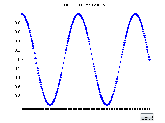
disp('f(x) = cos(x) on [0,9*pi/2]')
f = @(x) cos(x);
a = 0; b = 9*pi/2;
tol = 1.e-6;
q = quadgui(f,a,b,tol);

%pause
f(x) = cos(x) on [0,9*pi/2]
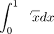
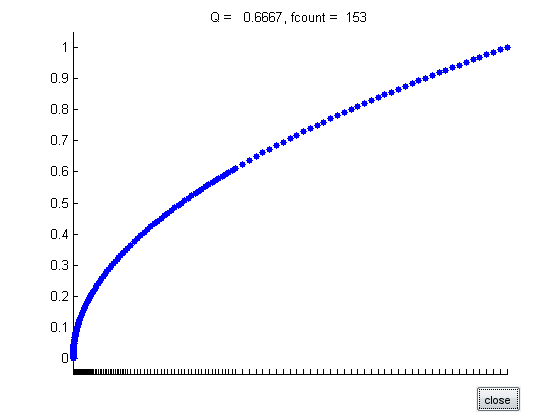
disp('f(x) = sqrt(x) on [0,1]')
f = @(x) sqrt(x);
a = 0; b = 1;
tol = 1.e-8;
q = quadgui(f,a,b,tol);

%pause
f(x) = sqrt(x) on [0,1]
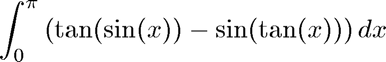
disp('f(x) = tan(sin(x))-sin(tan(x)) on [0,pi]')
f = @(x) tan(sin(x))-sin(tan(x));
a = 0; b = pi;
q = quadgui(f,a,b);
f(x) = tan(sin(x))-sin(tan(x)) on [0,pi]