SkydiveChuteDemo.m
Contents
Overview
This script illustrates the solution of a first-order IVP:
where  if
if  and
and  for
for  .
.
The analytical solution is

for finding the velocity of a skydiver when his parachute opens midflight. Here  stands for time,
  for velocity, and
 : gravitational constant
 : mass
 : (time dependent) drag coefficient
The analytical solution is coded in VelocityChute.m and the right-hand side function is coded in SkydiveChute.m
The Main Function
function SkydiveChuteDemo()
% Note that you cannot include other functions inside a *script*, but if
% you turn your main script into a *function*, then you can do it (see
% below).
Initialization
clear all
clc
close all
g = 9.81; m = 68.1; c1 = 10; c2 = 50;     % specific constants
v = @VelocityChute;                       % analytical solution
f = @SkydiveChute;                        % function handle for right-hand side function
t0 = 0; y0 = 0;                           % initial time and initial velocity
tend = 20;                                % end time
N = 100;                                  % number of time steps
h = (tend-t0)/N;                          % stepsize
Call Euler
We will discuss this function later
[t,y] = Euler(t0,y0,f,h,N);
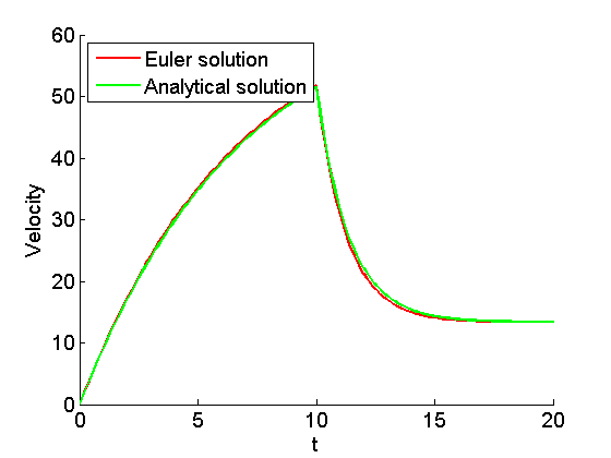
Plot
figure
hold on
set(gca,'Fontsize',14)
xlabel('t','FontSize',14);
ylabel('Velocity','FontSize',14);
plot(t,y,'r','LineWidth',2);              % Euler solution
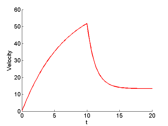
tt=linspace(t0,tend,201);
plot(tt,v(tt),'g','LineWidth',2);         % analytical solution
legend('Euler solution','Analytical solution','Location','NorthWest');
hold off
fprintf('Final velocity: %f m/s.', g*m/c2)
end
The VelocityChute Function
function v = VelocityChute(t)
% v = VelocityChute(t)
% t (time) is a vector of times at which we want to evaluate the analytical
% solution.
%
% v (velocity) is a vector with values of the analytical function.
%
% Note how we use *logical vectors* below to distinguish between the two
% cases (before and after the chute opens at time T).
%
% The following parameters are rough estimates
g = 9.81;  % gravitational constant (in m/s^2)
c1 = 10;   % drag coefficient (in kg/s)
c2 = 50;   % drag coefficient (in kg/s)
m = 68.1;  % mass of skydiver (in kg)
T = 10;    % time the chute opens
v1 = (g*m/c1 * (1-exp(-c1/m*t)));    % velocity if t < T
v2 = (g*m/c2 - g*m/(c1*c2) * exp(-c2/m*(t-T)) .* (c1-c2+c2*exp(-c1/m*T)));  % velocity if t >= T
v = v1 .* (t<T) + v2 .* (t>=T);    % multiplication by logical vectors here
end
Final velocity: 13.361220 m/s.
The SkydiveChute Function
function yprime = SkydiveChute(t,y)
% yprime = Skydive(t,y)
% t (time) and y (velocity v(t)) are scalars.
%
% yprime is the derivative of y at time t.
%
% The following parameters are rough estimates
g = 9.81;  % gravitational constant (in m/s^2)
c1 = 10;   % drag coefficient (in kg/s)
c2 = 50;   % drag coefficient (in kg/s)
m = 68.1;  % mass of skydiver (in kg)
T = 10;    % time the chute opens
if t < T
    yprime = g - (c1/m)*y ;
else
    yprime = g - (c2/m)*y ;
end
end