TwoBodyDemo.m
Contents
Overview
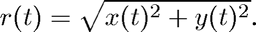
This script illustrates the use of ode23tx for the solution of the two-body problem
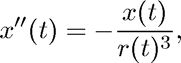
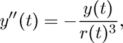
where
Here  and
and  are the coordinates of a small body (such as a space ship) relative to a (fixed) large body (such as a planet), and
  is time. In other words, the parametric curve
 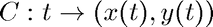 describes the orbit of the small body around the large body.
In order to apply an IVP solver we need to convert the system of two second-order ODEs to a system of four first-order ODEs, i.e.,
![$$ \mathbf{y} = \left[y_1, y_2, y_3, y_4 \right]^T = \left[x, x',
y, y' \right]^T $$](TwobodyDemo_eq95503.png)
so that
![$$ \mathbf{y}' = \left[y'_1, y'_2, y'_3, y'_4 \right]^T =
\left[y_2, -\frac{y_1}{r^3}, y_4, -\frac{y_3}{r^3} \right]^T $$](TwobodyDemo_eq38230.png)
This first-order system is coded in the function twobody.m.
Beginning of code
Initialize
clear all
close all
Example 1
Use ode23tx to solve the two-body problem with initial condition

i.e., with the small body starting at  with unit initial velocity in the "upward" direction. The large body is to be interpreted as a point mass located at the origin. We use a time interval of
 ![$[0,2\pi]$](TwobodyDemo_eq96599.png) . The horizontal axis in the plot is the -axis. The different colors correspond to
. The horizontal axis in the plot is the -axis. The different colors correspond to
- dark blue:
 (identical with
  )
) - green:

- red:

- light blue:
ode23tx(@twobody,[0 2*pi],[1; 0; 0; 1]);
pause
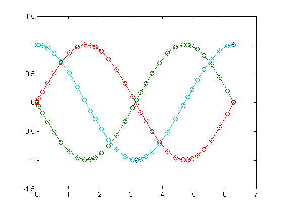
To get a phase plane plot, i.e., a plot of the -parametrized actual orbit determined by the first and third components of the system of four first-order ODEs we store the output of ode23tx in t and y and then plot those first and third components of y together.
y0 = [1; 0; 0; 1];
[t,y] = ode23tx(@twobody,[0 2*pi],y0);
plot(y(:,1),y(:,3),'-',0,0,'ro')
xlabel('x'), ylabel('y')
axis equal
pause
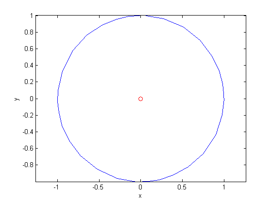
Example 2
Now we use ode23tx to solve the two-body problem with slightly modified initial conditions

i.e., we increase the initial velocity in the "upward" direction. We also change the time interval to ![$[0,12\pi]$](TwobodyDemo_eq82391.png) . Again, the horizontal axis in the plot is the -axis, and the different colors correspond to
. Again, the horizontal axis in the plot is the -axis, and the different colors correspond to
- dark blue:
- green:
- red:
- light blue:
y0 = [1; 0; 0; 1.3];
ode23tx(@twobody,[0 12*pi],y0);
pause
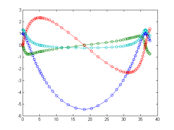
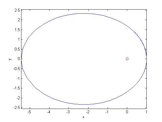
The corresponding phase plane plot for this modified -velocity is given by
y0 = [1; 0; 0; 1.3];
[t,y] = ode23tx(@twobody,[0 12*pi],y0);
plot(y(:,1),y(:,3),'-',0,0,'ro')
xlabel('x'), ylabel('y')
axis equal